We wish to detect regions of stability and uncertainty in the financial markets of Spain during the 2008 crisis. These may be interpreted to detect the start of the crisis. We will use a Bayesian approach implemented in Stan and interfaced in R.
Bayesian model: Markovian regime switching
We consider a time series \(y = (y_t)\) whose behaviour at each instant depends on the state at which we are. We assume there are 2 such states and at each instant we can be in either, resulting in another time series \(z = (z_t), \ z_t \in \{ 1, 2\}\).
The model is characterized by \(z_t\) being a Markov chain. This is expressed by
\[p(z_t = k \mid z_{t-1} = i) := \begin{cases} p_{ki}, & k = i \\ 1 - p_{ki}, & k \neq i \end{cases} , \quad \text{ for }i,k\in\{1,2\}.\]Finally, we consider that \(y_t\) is an autoregressive process of order \(p\). That is,
\[y_t \mid z_t = k, \mathbf{Y}_t, \theta \sim \mathcal{N}(\mu_k + \mathbf{c}_k^\top \mathbf{Y}_t, \sigma_k).\]Note that \(\mathbf{Y}_t\) is a lag vector containing the previous \(p\) observations of \(y\), and \(\mathbf{c}_k\) contains the coefficients of the autoregression (for each state \(k \in \{1,2\}\)). In other words, \(f(y_t \mid z_t = k, \textbf{Y}_t, \theta) = \frac{1}{\sigma_k \sqrt{2 \pi }} \mathrm{exp}\left(-\frac{\left(y_t - \mu_k - \mathbf{c}_k^\top \mathbf{Y}_t\right)^2}{2 \sigma_k ^2}\right)\).
Distribution function
We consider the set of parameters \(\Theta = (\pi_1, \pi_2, p_{11}, p_{22}, \mu_1, \mu_2, \mathbf{c}_1, \mathbf{c}_2, \sigma_1, \sigma_2)\). Here, \(\pi_1, \pi_2\) denote the probability of being in state 1 or 2 at \(t=p+1\). Then, due to the autoregressive function, we may express
\[p(y, z \mid \Theta) = \pi_{z_{p+1}} f (y_{p+1} \mid z_{p+1}, \mathbf{Y}_{p+1}, \Theta) \prod_{t = p+2}^n p(z_t \mid z_{t-1}) f(y_t \mid z_t, \mathbf{Y}_{t}, \Theta).\]We wish to marginalize over \(z\) to obtain a distribution function of the single observable \(y\). However, doing so in a naive way involves summing over \(2^{N-1}\) terms (N being the length of the series), which is very inefficient.
Forward algorithm
We will use the recurrence character to obtain the marginalized distribution. Define \(\alpha_t(k) = p(y_{[1,t]}, z_t = k)\). We then have:
\[\begin{cases} \alpha_{p+1}(k) = \pi_k f(y_{p+1} \mid z_{p+1} = k, \Theta) \\ \alpha_t(k) = \left[ \sum_{i=1}^2 p_{ki} \alpha_{t-1}(i) \right] f(y_t \mid z_t = k) \end{cases} .\]This way, the distribution function for \(y_{[1,t]}\) having marginalized \(z\) is simply
\[p(y_{[1,t]}) = \alpha_t(1) + \alpha_t(2).\]Log likelihood function
By defining \(l_t(k) = \log(\alpha_t(k))\), we have the recurrence
\[\begin{cases} l_{p+1}(k) = \log{\pi_k} + \log{f(y_{p+1} \mid z_{p+1} = k, \textbf{Y}_{p+1}, \Theta)} \\ l_{t}(k) = \log{\left[ \sum_{i=1}^2 \mathrm{exp}(l_{t-1}(k) + \log{p_{ki})} \right] } + \log{f(y_{t} \mid z_{t} = k, \textbf{Y}_t, \Theta)} \\ \end{cases}.\]Then, the logarithm of the likelihood function \(\mathcal{L}_y (\Theta) = \log(p(y_{[1,N]} \mid \Theta))\) is
\[\mathcal{L}_y (\Theta) = \log{\left(\alpha_N(1) + \alpha_N(2)\right)} = \log{\left[\mathrm{exp}(l_N(1)) + \mathrm{exp}(l_N(2))\right]}.\]Regime probability
Note that at each instant of time, we can compute \(\xi_t (k) = p (z_t = k \mid y_{[1,t]})\). We have
\[\xi_t(k) = \frac{\alpha_t(k)}{\alpha_t(1) + \alpha_t(2)}.\]Data
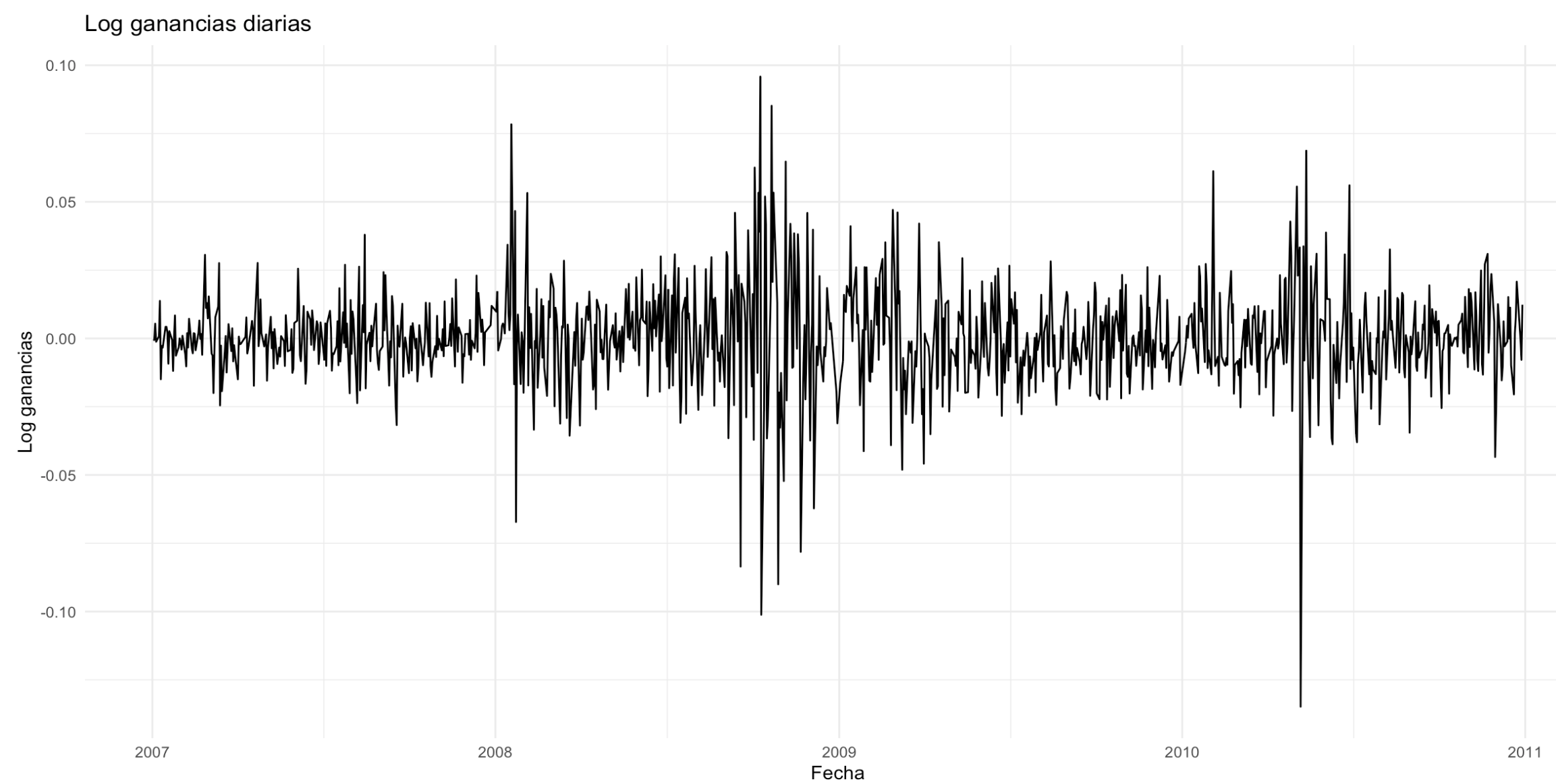
We will use the values of the IBEX35 index from 2007 to 2011. In particular, at each day, we compute the log intraday return
\[y_t := \log{(\frac{P_{t, \text{close}}}{P_{t, \text{open}}})} = \log{P_{t, \text{close}}} - \log{P_{t, \text{open}}}.\]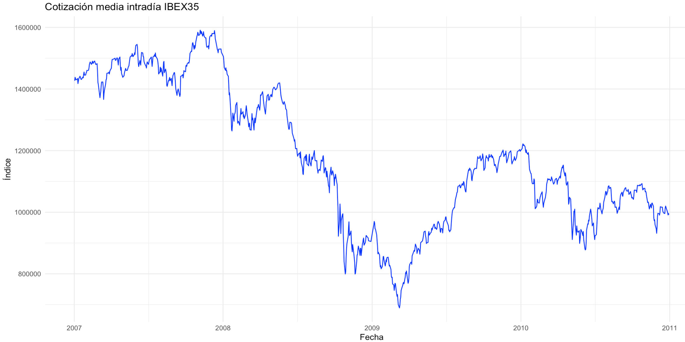
R and Stan implementation
We have used Stan to implement the model. Recall that we have a total of \(6 + 2p\) parameters, after fixing \(\pi_1 = \pi_2 = 1 / 2\) for simplicity. That is \(\mu_0, \mu_1 \in \mathbb{R}, \ \sigma_0, \sigma_1 \in (0, \infty), \ p_{11}, p_{22} \in (0,1), \ \mathbf{c}_1, \mathbf{c}_2 \in \mathbb{R}^p\).
Prior distributions
The priors bias \(p_{11}, p_{22}\) toward persistence (\(\approx 1\)), making regime changes rare. Means are constrained with \(\mu_0 > \mu_1\), so regime 0 reflects more gains (no crisis) than regime 1 (crisis). Volatility is higher in the crisis state, enforced via both constraints and weaker priors. AR coefficients are shared across regimes, but the first lag has higher prior variance to allow stronger influence from the previous day.
| Variable | Distribution | Constraints | Parameters |
|---|---|---|---|
| \(p_{11}, p_{22}\) | \(\mathrm{Beta}(a, b)\) | – | \((a,b) = (10, 2)\) |
| \(\mu_0\) | \(\mathcal{N}(a_0, b^2_0)\) | – | \((a_0, b_0) = (0.01, 0.02)\) |
| \(\mu_1\) | \(\mathcal{N}(a_1, b^2_1)\) | \(\mu_1 < \mu_0\) | \((a_1, b_1) = (-0.01, 0.02)\) |
| \(\sigma_0\) | \(\mathrm{Cauchy}(r_0, s_0)\) | \(\sigma_0 > 0\) | \((r_0, s_0) = (0, 0.2)\) |
| \(\sigma_1\) | \(\mathrm{Cauchy}(r_1, s_1)\) | \(\sigma_1 > \sigma_0\) | \((r_1, s_1) = (0, 1)\) |
| \(c_{ki}, \quad k \in \{1,2\}, \; i \in [1:p-1]\) | \(\mathcal{N}(m_{ki}, n^2_{ki})\) | – | \((m_{k1}, n_{k1}) = (0, 0.2)\) \((m_{ki}, n_{ki}) = (0, 0.1), \; i \in [2:p-1]\) |
Stan code
data {
	int<lower=1> N;              // number of observations (after lags)
	int<lower=1> p;              // AR order
	matrix[N, p] Ylag;           // lagged design matrix
	vector[N]    y;              // response vector
}

parameters {
	vector<lower=0,upper=1>[2]  p_trans;   // p_trans[1]=P(stay in state 1), p_trans[2]=P(stay in state 2)
	real                        mu0;
	real<upper=mu0>             mu1;
	vector[p]                   c0;
	vector[p]                   c1;
	real<lower=0>               sigma0;
	real<lower=sigma0>          sigma1;
}

transformed parameters {
	// total log-likelihood via forward algorithm
	real        log_lik;
	vector[2]   log_alpha_prev;
	vector[2]   log_alpha_curr;

	// initialize
    real p1_init = 1.0/2.0;
    log_alpha_prev[1] = log(p1_init);
    log_alpha_prev[2] = log1m(p1_init);

	// forward pass
	for (t in 1:N) {
		real le1 = normal_lpdf(y[t] | mu0 + dot_product(Ylag[t], c0), sigma0);
		real le2 = normal_lpdf(y[t] | mu1 + dot_product(Ylag[t], c1), sigma1);
		for (k in 1:2) {
			vector[2] temp;
			// transition from state i to k
			temp[1] = log_alpha_prev[1] + log(k == 1 ? p_trans[1] : (1 - p_trans[1]));
			temp[2] = log_alpha_prev[2] + log(k == 2 ? p_trans[2] : (1 - p_trans[2]));
			log_alpha_curr[k] = log_sum_exp(temp) + (k == 1 ? le1 : le2);
		}
		log_alpha_prev = log_alpha_curr;
	}
	// total marginal likelihood
	log_lik = log_sum_exp(log_alpha_curr);
}

model {
    p_trans ~ beta(10, 2);
    mu0     ~ normal(0.01, 0.02);
    mu1     ~ normal(-0.01, 0.02);
    c0[1]   ~ normal(0, 0.2);
    c1[1]   ~ normal(0, 0.2);
    for (j in 2:p) {  // Additional lags with lower value
        c0[j] ~ normal(0, 0.1);
        c1[j] ~ normal(0, 0.1);
    }
    sigma0 ~ cauchy(0, 0.2);
    sigma1 ~ cauchy(0, 1);

	target += log_lik;
}

generated quantities {
	matrix[N,2] xi;          // filtered state probabilities
	vector[2]   alpha_fwd;
	vector[2]   new_alpha;

	// initialize forward probabilities at stationarity
    alpha_fwd[1] = p1_init;
    alpha_fwd[2] = 1 - p1_init;

	for (t in 1:N) {
		// recompute emission densities
		real e1 = exp(normal_lpdf(y[t] | mu0 + dot_product(Ylag[t], c0), sigma0));
		real e2 = exp(normal_lpdf(y[t] | mu1 + dot_product(Ylag[t], c1), sigma1));

		// one-step predict and update
		new_alpha[1] = (alpha_fwd[1] * p_trans[1] + alpha_fwd[2] * (1 - p_trans[2])) * e1;
		new_alpha[2] = (alpha_fwd[1] * (1 - p_trans[1]) + alpha_fwd[2] * p_trans[2]) * e2;

		// normalize to get filtered probability
		xi[t,] = (new_alpha / sum(new_alpha))';
		alpha_fwd = (xi[t,])';
	}
}
Results
We fixed \(p = 5\). Launching 4 chains with 4000 iterations and a warm-up of 1000 iterations, Stan converged successfully to the corresponding posterior distributions which we do not show here.
We do show however the probability of being in each state at each instant of time.
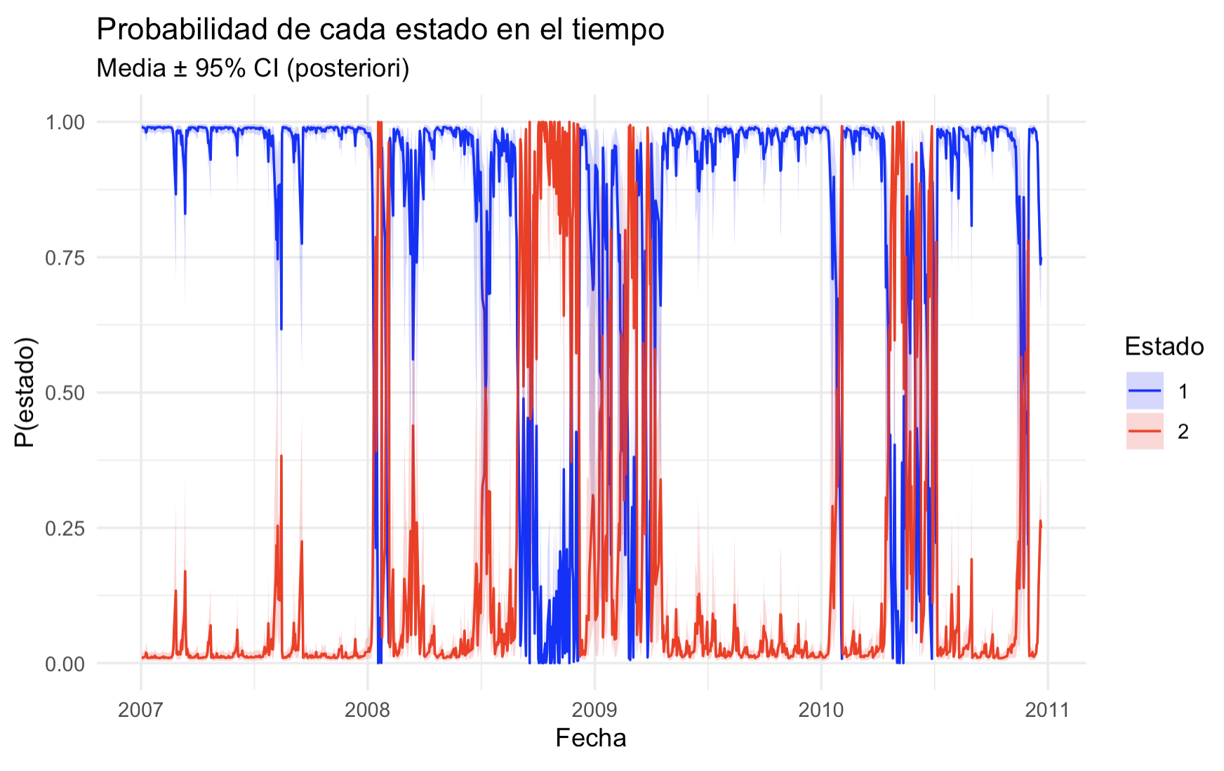
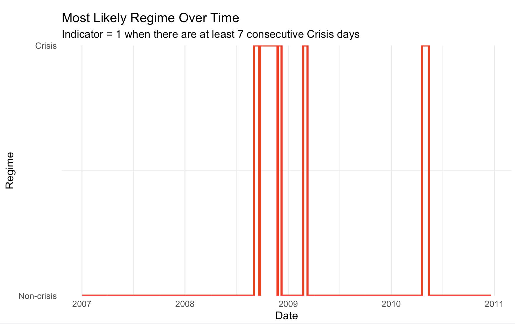
We may treat these results to obtain an indicator variable for crisis or instability periods.
Hierarchical model
We have also implemented a hierarchical model to compare results on the behaviour of some representative companies of each sector. This is not shown here.