Exact symplectomorphisms and an application to convex billiards
In this work, which was the final project for the Hamiltonian systems course of my Master’s, we first explore some properties of exact symplectomorphisms, with the ultimate goal of establishing a relationship between the critical points of their generating function and the fixed points of the corresponding discrete dynamical map. To this end, notions of differential geometry are developed, and we use variational methods (generalized Lagrange multipliers) to obtain the main results. In the second part, we briefly focus on the Billiard map and study it from the point of view of the theory developed previously. In particular, we give a precise meaning to its generating function and see how this allows us to establish the existance of periodic orbits. Finally, this framework allows us to understand the length spectrum from a symplectic point of view.
Exact symplectomorphisms
In this chapter we introduce symplectic geometry, and dive into some properties of primitive functions of exact symplectomorphisms. By the end we relate some of the dynamics of such maps with their primitive functions via some variational principles.
Preliminaries: Transversality and Lagrange multipliers
In this subsection we present some results that will be used in the development of the chapter, in particular, regarding regular values of maps and the method of Lagrange multipliers in manifolds. We will not prove these results, but their proofs can be found in [@abraham2012manifolds].
A function \(f \colon \mathcal{M} \to \mathcal{N}\) is called an immersion if \(\mathrm{d}f_p\) is injective \(\forall p \in \mathcal{M}\). That is, if \(\mathrm{rank}(Df) = \mathrm{dim}(\mathcal{M})\).
A function \(f \colon \mathcal{M} \to \mathcal{N}\) is called a submersion if \(\mathrm{d}f_p\) is surjective \(\forall p \in \mathcal{M}\). That is, if \(\mathrm{rank}(Df) = \mathrm{dim}(\mathcal{N})\).
A point \(n \in \mathcal{N}\) is a regular value of \(f\) if \(\forall p \in f^{-1}(\mathcal{N}), \ \mathrm{d}f_p\) is surjective. That is, if all the points of the preimage of \(n\) are regular points of f.
The following is a useful theorem we will not prove.
(Regular value theorem) Let \(f \colon \mathcal{M} \to \mathcal{N}\) be a smooth map between smooth manifolds. For every regular value \(y \in \mathcal{N}\), \(S=f^{-1}(y)\) is either \(\emptyset\) or a smooth submanifold of \(\mathcal{M}\) with \(\mathrm{dim}(S) = \mathrm{dim}(N) - \mathrm{dim}(M)\) and \(T_x S \cong \mathrm{ker}(\mathrm{d}f)_x\).
A mapping \(f \colon \mathcal{M} \to \mathcal{N}\) is transversal to the submanifold \(\mathcal{Z} \subset \mathcal{N}\) if the transversality equation \(\mathrm{Im}(\mathrm{d}f_x) + T_y \mathcal{Z} = T_y \mathcal{N}\) holds at every \(x = f^{-1}(y) \in f^{-1}(\mathcal{Z})\). We denote it as \(f \pitchfork \mathcal{Z}\).
If each point of \(\mathcal{Z}\) is a regular value of \(f\), then \(f \pitchfork \mathcal{Z}\).
If \(f\) is the inclusion map \(i \colon \mathcal{M} \to \mathcal{N}\), the transversality equation becomes \(T_x \mathcal{M} + T_{x} \mathcal{Z} = T_x \mathcal{N}\)
The following is a generalization of the regular value theorem.
Let \(f \colon \mathcal{M} \to \mathcal{N}\) smooth, \(\mathcal{Z}\) a submanifold of \(\mathcal{N}\). If \(f \pitchfork \mathcal{Z}\), then \(f^{-1}(\mathcal{Z})\) is a submanifold of \(\mathcal{M}\), and \(\mathrm{codim}_{\mathcal{M}}(f^{-1}(\mathcal{Z})) = \mathrm{codim}_{\mathcal{N}}(Z)\).
A fact about transversal submanifolds is that if \(f\) is transversal to two submanifolds of \(\mathcal{M}\), then it is also transversal to their intersection.
We now have all the pieces to state the generalized Lagrange multipliers theorem and a useful corollary.
(Lagrange multipliers) Let \(g \colon \mathcal{M} \to \mathcal{P}\) be a smooth map, \(p \in P\) a regular value of \(g\), \(\mathcal{N} = g^{-1}(p)\), and \(f \colon \mathcal{M} \to \mathbb{R}\) be \(\mathcal{C}^r, r \geq 1\). Then, a point \(n \in \mathcal{N}\) is a critical point of \(f|_N\) if \(\exists \lambda \in T_p^* \mathcal{P}\) such that \(\mathrm{d}f_n = \lambda \circ \mathrm{d}g_n\). We call \(\lambda\) a Lagrange multiplier.
A similar result holds when \(\mathcal{N}\) is the preimage of a transversal manifold of \(g\), not just a regular value.
Let \(g \colon \mathcal{M} \to \mathcal{P}\) smooth, \(\mathcal{Z}\) a submanifold of \(P\). Suppose \(g \pitchfork \mathcal{Z}\), and let \(\mathcal{N} = g^{-1} (\mathcal{Z})\). Let \(f \colon \mathcal{M} \to \mathbb{R}\) be \(\mathcal{C}^r, r \geq 1\). Let \(E_{g(n)}\) be a closed component to \(T_{g(n)}\mathcal{Z}\) in \(T_{g(n)}\mathcal{P}\), so we have \(T_{g(n)} \mathcal{P} = T_{g(n)} \mathcal{Z} \oplus E_{g(n)}\), with \(\pi \colon T_{g(n)}\mathcal{P} \to E_{g(n)}\) the projection. Then a point \(n \in \mathcal{N}\) is a critical point of \(g|_{\mathcal{N}}\) if \(\exists \lambda \in E^*_{g(n)}\) such that \(\mathrm{d}f_n = \lambda \circ \pi \circ \mathrm{d}g_n\).
Note that in the previous corollary, \(E_{g(n)}\) can be interpreted as the normal component to \(\mathcal{Z}\) in \(\mathcal{P}\).
Symplectic manifolds
A 2-form \(w\) on a manifold \(\mathcal{M}\) is a symplectic form if it is closed (\(\mathrm{d}w = 0\)) and nondegenerate (\(\forall \alpha \ \text{1-form}, \ \exists ! X \ \text{vector field on} \ M \ \text{s.t.} \ \iota_X w = \alpha\)).
Note that \(\mathrm{d}\) is the exterior derivative and \(\iota_X w\) is the contraction or interior product of \(w\) with \(X\). Since the 2-form is nondegenerate, the dimension of a symplectic manifold must be even \(\mathrm{dim}(\mathcal{M}) = 2n\). Another consequence is that it has a canonical volume form \(w^n\), and hence \(\mathcal{M}\) must be orientable.
A symplectic manifold is a pair \((\mathcal{M}, w)\) such that \(\mathcal{M}\) is a differential manifold and \(w\) is a symplectic form on \(\mathcal{M}\).
\(\mathcal{M}= \mathbb{R}^{2n}\) with linear coordinates \(x_1, \ldots, x_n, y_1, \ldots, y_n\) and the form \(\mathrm{d}x \wedge \mathrm{d}y = \sum_{i=1}^n \mathrm{d}x_i \wedge \mathrm{d}y_i\) is a symplectic manifold.
Let \((\mathcal{M}_1, w_1)\), \((\mathcal{M}_2, w_2)\) be \(2n\)-dimensional symplectic manifolds, and \(\varphi \colon \mathcal{M}_1 \to \mathcal{M}_2\) a diffeomorphism. We say that \(\varphi\) is a symplectomorphism if \(\varphi^* w_2 = w_1\).
Recall that by definition of pullback, \(\varphi^* w_2 = w_1\) is the same as saying that for vectors \(u,v \in T_p \mathcal{M}_1\) we have that \((w_1)_p (u,v) = (w_2)_{\varphi(p)}(\mathrm{d} \varphi_p(u), \mathrm{d} \varphi_p(v))\).
Classification of symplectic manifolds up to symplectomorphism, at least locally, is a consequence of the following theorem. It turns out that just as any \(n\) dimensional smooth manifold is locally diffeomorphic to \(\mathbb{R}^n\), any \(2n\)-symplectic manifold is locally symplectomorphic to \((\mathbb{R}^{2n}, w_0)\), so the only local invariant is the dimension.
(Darboux’s) Let \((\mathcal{M}, w)\) be a symplectic manifold, and \(p \in \mathcal{M}\). Then there is a coordinate chart \((\mathcal{U}, x_1, \ldots, x_n, y_1, \ldots, y_n)\) centered at \(p\) such that, on \(\mathcal{U}\), \(w = \mathrm{d}x \wedge \mathrm{d}y = \sum_{i=1}^n \mathrm{d}x_i \wedge \mathrm{d}y_i\).
This chart is called a Darboux chart, and the theorem implies that symplectic manifolds are all locally symplectomorphic to \((\mathbb{R}^{2n}, w_0)\). Note that by the Poincaré lemma, locally there always exists a 1-form \(\alpha\) such that \(\mathrm{d}\alpha = w\). In local coordinates \((x,y)\), \(\alpha = -y \mathrm{d}x\).
Canonical symplectic form on the cotangent bundle
Let \(\mathcal{X}\) be a smooth manifold of dimension \(n\), and let \(\mathcal{M} = T^* \mathcal{X}\) be its cotangent bundle. Let \((\mathcal{U}, x_1, \ldots, x_n)\) be a coordinate chart for \(\mathcal{U} \subset \mathcal{X}\), and \((T^* \mathcal{U}, x_1, \ldots, x_n, \xi_1 , \ldots, \xi_n)\) be the induced coordinate chart on \(T^* \mathcal{U} \subset \mathcal{M}\), so if \(p \in \mathcal{U}\) then \(\xi \in T^*_p \mathcal{U}\) can be expressed as \(\xi = \sum_{i=1}^n \xi_i (\mathrm{d}x_i)_p\).
The tautological 1-form or Liouville form on \(T^* \mathcal{U}\) is \(\alpha = \sum_{i=1}^n \xi_i \mathrm{d}x_i\).
The canonical symplectic form on \(T^* \mathcal{U}\) is \(w = -\mathrm{d} \alpha\), so \(w = \mathrm{d}x \wedge \mathrm{d} \xi = \sum_{i=1}^n \mathrm{d}x_i \wedge \mathrm{d} \xi_i\).
It can be checked that these forms are intrinsically defined, so they do not depend on the coordinate charts.
To give an intepretation to the Liouville form, it may be useful to give an alternative coordinate free definition. Let \(\pi \colon T^*\mathcal{X} \to \mathcal{X} \colon p = (x, \xi) \to x\) be the natural projection. Then, \(\alpha_p = \xi \circ \mathrm{d} \pi_p\). Note that \(\mathrm{d}\pi_p \colon T_p(T^*\mathcal{X}) \to T_{\pi (\rho)} \mathcal{X}\). Then, we say that the value of \(\alpha\) on a vector \(v \in T_{(x, \xi)} ( T^*\mathcal{X})\) is equal to the value of the 1-form \(\xi\) on the projection of \(v\) to the tangent space \(T_x \mathcal{X}\). It is called tautological because it naturally identifies the evaluation of \(\xi\) on vectors tangent to \(\mathcal{X}\).
Moreover, \(\alpha\) is the unique 1-form on \(\mathcal{M}\) satisfying \(\rho^* \alpha = \rho, \ \forall \rho \in \Omega^1(\mathcal{M})\).
There are more general symplectic manifolds with the property that \(w = \mathrm{d} \alpha\) for some 1-form \(\alpha\), not just cotangent bundles.
A symplectic manifold \((\mathcal{M}, w)\) is called exact if \(\exists\) a 1-form \(\alpha\) such that \(w = \mathrm{d} \alpha\).
An interesting result is that exact symplectic manifolds cannot be compact and without a boundary.
Exact symplectomorphisms and primitive functions
A symplectomorphism \(F \colon \mathcal{M} \to \mathcal{M}\) on an exact symplectic manifold \((\mathcal{M}, \mathrm{d}\alpha)\) is called exact if \(\exists\) a function \(S \colon \mathcal{M} \to \mathbb{R}\) such that \(F^* \alpha - \alpha = \mathrm{d}S\). \(S\) is the generating function or primitive function of \(F\), denoted as \(\mathrm{pf}(F) = S\).
Note that \(\mathrm{pf}(F) = S\) is defined up to an additive constant.
A symplectomorphism \(F \colon \mathcal{M} \to \mathcal{M}\) on an exact symplectic manifold \((\mathcal{M}, \mathrm{d}\alpha)\) is called an actionmorphism if \(F^* \alpha = \alpha\).
Composition formulae
We now propose some useful formulae to compute primitive functions of different combinations of exact symplectomorphisms.
Let \((\mathcal{M}, \mathrm{d}\alpha)\) be an exact symplectic manifold, and \(F, G \colon \mathcal{M} \to \mathcal{M}\) two exact symplectomorphisms with \(\mathrm{pf}(F) = S\), \(\mathrm{pf}(G) = T\). Then, up to an additive constant:
-
\(\mathrm{pf}(G \circ F) = \mathrm{pf}(F) + \mathrm{pf}(G) \circ F = S + T \circ F\).
-
\(\mathrm{pf}(F^{-1}) = -\mathrm{pf}(F) \circ F^{-1} = -S \circ F^{-1}\).
- \[\begin{aligned} \mathrm{pf}(G^{-1} \circ F \circ G) &= \mathrm{pf}(F) \circ G + \mathrm{pf}(G) - \mathrm{pf}(G)\circ G^{-1} \circ F \circ G \\ &= S \circ G + T - T \circ G^{-1} \circ F \circ G. \end{aligned}\]
Proof
A simple computation using properties of the pullback gives \((G \circ F)^* \alpha = F^* \circ G^* \alpha = F^* (\alpha + \mathrm{d}T) = F^* \alpha + F^* \mathrm{d}T = (\alpha + \mathrm{d}S) + \mathrm{d}(F^* T) = \alpha + \mathrm{d}S + \mathrm{d}(T \circ F)\), directly implying the first identity: \((G \circ F)^* \alpha - \alpha = \mathrm{d}(S + T \circ F)\).
For the second identity, let \(G = F^{-1} \circ F^{-1}\) and use the
previous identity two times:
\(\mathrm{pf}(F^{-1}) = \mathrm{pf}(G \circ F) = S + \mathrm{pf}(F^{-1} \circ F^{-1})\circ F = S + \left[\mathrm{pf}(F^{-1}) + \mathrm{pf}(F^{-1})\circ F^{-1} \right]\circ F = S + \mathrm{pf}(F^{-1}) \circ F + \mathrm{pf}(F^{-1}) \implies \mathrm{pf}(F^{-1})\circ F = -S\).
For the third, let \(\hat F = G, \ \hat G = G^{-1} \circ F\), and use both identities: \(\mathrm{pf}(G^{-1} \circ F \circ G) = \mathrm{pf}(\hat G \circ \hat F) = \mathrm{pf}(\hat F) + \mathrm{pf}(\hat G) \circ \hat F = \mathrm{pf}(G) + \left[ \mathrm{pf}(F) + \mathrm{pf}(G^{-1}) \circ F \right] \circ G = T + S \circ G - T \circ G^{-1} \circ F \circ G\). ◻
As a small parenthesis, this allows us to prove an interesting fact about primitive functions. In particular, that given a primitive function the corresponding symplectomorphism is not uniquely determined. This is why we prefer to call them primitive functions and not generating functions.
Let \((\mathcal{M}, \mathrm{d}\alpha)\) be an exact symplectic manifold, and \(F \colon \mathcal{M} \to \mathcal{M}\) an exact symplectomorphism with \(\mathrm{pf}(F) = S\). Then, \(F\) is determined by \(S\) up to actionmorphisms by the left, i.e., \(\{ G \mid \mathrm{pf}(G) = S\} = \{ L \circ F \mid \mathrm{pf}(L) = 0\}\).
Proof
Let \(G\) s.t. \(\mathrm{pf}(G) = S\). Define \(L = G \circ F^{-1}\). Then, by [prop:composition], \(\mathrm{pf}(L) = \mathrm{pf}(G \circ F^{-1}) = \mathrm{pf}(F^{-1}) + \mathrm{pf}(G) \circ F^{-1} = -S \circ F^{-1} + S \circ F^{-1} = 0\). ◻
In order to completely determine \(F\) from \(S\) we need additional information. Details can be found in [A. HARO PHD].
Now we consider the action of \(F^n\).
Let \((\mathcal{M}, \mathrm{d}\alpha)\) be an exact symplectic manifold, and \(F \colon \mathcal{M} \to \mathcal{M}\) an exact symplectomorphism with \(\mathrm{pf}(F) = S\). Then, \(\mathrm{pf}(F^n) = \sum_{i=0}^{n-1} S \circ F^i\).
Proof
By induction. The base case is simply \(\mathrm{pf}(F) = S\). The induction hypothesis is that \(\mathrm{pf}(F^{n-1}) = \sum_{i=0}^{n-2}S \circ F^i\). Now, use [prop:composition] on \(\mathrm{pf}(F^n) = \mathrm{pf}(F \circ F^{n-1})\), and we have that
\(\mathrm{pf}(F \circ F^{n-1}) = \mathrm{pf}(F^{n-1}) + \mathrm{pf}(F) \circ F^{n-1} = \sum_{i=0}^{n-2}S \circ F^i + S \circ F^{n-1} = \sum_{i=0}^{n-1}S \circ F^i\). ◻
This result allows for the definition of an intrinsic quantity of periodic orbits of the symplectomorphism \(F\) as we will discuss in section 1.6.
Symplectic product
Given \(n\) symplectic manifolds, we wonder about the nature of their direct product.
Given \((\mathcal{M}_1, w_1), \ldots, (\mathcal{M}_n, w_n)\) a collection of \(n\) symplectic manifolds, then their direct product \(\mathcal{M} = \mathcal{M}_1 \times \ldots \times \mathcal{M}\) is a symplectic manifold with symplectic form \(\Omega = \sum_{i=1}^q \pi_i^* w_i\), with \(\pi_i \colon \mathcal{M} \to \mathcal{M}_i\) the projection map. Moreover, if they are exact with \(w_i = \mathrm{d} \alpha_i\), then \(\mathcal{M}\) is also exact with \(\Omega = \mathrm{d}A\), \(A = \sum_{i=1}^q \pi_i^* \alpha_i\).
In this manner we can also define a symplectomorphism on the direct product given a collection of symplectomorphisms on the original manifolds.
Consider the product of \(n\) exact symplectic manifolds \(\mathcal{M} = \prod_{i=1}^{q} \mathcal{M}_i\), with symplectic form \(\Omega = \mathrm{d}A = \sum_{i=1}^q \pi_i^* \mathrm{d}\alpha_i\). Let \(F_i \colon \mathcal{M}_i \to \mathcal{M}_i\) be a collection of \(q\) exact symplectomorphisms with \(\mathrm{pf}(F_i) = S_i\). Then, \(F = F_1 \times \ldots \times F_q\) is an exact symplectomorphism on \(\mathcal{M}\), with \(\mathrm{pf}(F) = S = \sum_{i=1}^q S_i \circ \pi_i\).
This allows for an alternative view of periodic orbits using a parallel shooting approach.
Given a diffeomorphism \(F \colon \mathcal{M} \to \mathcal{M}\), we define on \(\mathcal{M}^q = \prod_{i=0}^{q-1} \mathcal{M}\) the diffeomorphism \(F_q \colon \mathcal{M}^q \to \mathcal{M}^q\), \(F_q(z_0, \ldots, z_{q-1}) = (F(z_{q-1}), F(z_0), \ldots, F(z_{q-2}))\). Then,
-
Fixed points of \(F_q\) are in correspondance with \(q\)-periodic points of \(F\) (\(q\)-to-1).
-
If \(F\) is exact with \(\mathrm{pf}(F) = S\), then \(F_q\) is also exact with \(\mathrm{pf}(F_q) = S_q \colon \mathcal{M}^q \to \mathbb{R}\), \(S_q(z_0, \ldots, z_{q-1}) = \sum_{i=0}^{q-1} S(z_i)\).
Action of periodic orbits
Given a \(q\)-periodic point \(z \in \mathcal{M}\) on an exact symplectic manifold of the exact symplectomorphism \(F\), we define the action along the orbit of \(z\) as \(S_q(z) = \mathrm{pf}(F^q)(z) = \sum_{i=0}^{q-1}S(F^i(z))\). The averaged action is then \(\hat S_q (z) = \frac{1}{q} S_q(z)\).
Note that \(S_q\) and \(\hat S_q\) are the same if we choose any other iterate of \(z\), and are thus unique for a particular periodic orbit. We now ask ourselves how this quantity changes if we perform a symplectic change of variables.
Recall that if we have a dynamical system given by a diffeomorphism \(F \colon \mathcal{M} \to \mathcal{M}\), i.e. \(x_{n+1} = F(x_n)\), and we perform a change of variables \(x = G(y)\), in the new variables we have that \(y_{n+1} = G^{-1}(F(G(y_n)))\). Thus, \(y_{n+1} = \bar F (y_n)\), with \(\bar F = G^{-1} \circ F \circ G\).
Let \((\mathcal{M}, \mathrm{d} \alpha)\) be an exact symplectic manifold, \(F \colon \mathcal{M} \to \mathcal{M}\) be an exact symplectomorphism. We conjugate \(F\) by another exact symplectomorphism \(G \colon \mathcal{M} \to \mathcal{M}\). Define \(\bar F = G^{-1} \circ F \circ G\). Then
2em there exists a constant \(C \in \mathbb{R}\) s.t. for all \(q\)-periodic points \(z \in \mathcal{M}\) of \(F\) (so \(\bar z = G^{-1} (z)\) is \(q\)-periodic of \(\bar F\)) the corresponding averaged actions differ by \(C\), \(\hat {\bar {S_q}}(\bar z) = \hat S_q(z) + C\).
Proof
Let \(\mathrm{pf}(F) = S\), \(\mathrm{pf}(G) = T\), \(\mathrm{pf}(\bar F) = \bar S\). By [prop:composition] we know that \(\bar S = S \circ G + T - T \circ \bar F + C\) for some \(C \in \mathbb{R}\). By definition, \({\bar{ S_q}}(\bar z) = \sum_{i=0}^{q-1} \left[ S(G(\bar F^i (z))) + T (\bar F^i(z)) - T (\bar F (\bar F^i (z))) + C\right] = qC + \sum_{i=0}^{q-1} \left[ S(G(\bar F^i (z))) + T(\bar F^i(z)) - T(\bar F^{i+1}(z))\right]\). Since we are at a periodic orbit, the last two terms will cancel out inside of the sum. Thus, \({\bar {S_q}}(\bar z) = qC + \sum_{i=0}^{q-1} S(G(\bar F^i (z)))\). Note that \(\bar F^i = G^{-1} \circ F^i \circ G\). Thus, \({\bar {S_q}}(\bar z) = qC + \sum_{i=0}^{q-1} S(G(G^{-1}(F^i(G(\bar z))))) = qC + \sum_{i=0}^{q-1} S(F^i(z)) = qC + S_q (z)\). ◻
We conclude that the average action of a periodic orbit is invariant under exact symplectic coordinate transformations, up to an additive constant that is precisely the constant of [prop:composition].
Variational principles in cotangent bundles
We will now present some interesting variational principles in the case where our symplectic manifold is a cotangent bundle. Equivalent results hold on the easier case of \(\mathbb{R}^{2n}\).
From now on, consider \(\mathcal{M}\) a manifold of dimension \(n\), and \(T^*\mathcal{M}\) its cotangent bundle. Recall that we can equip \(T^*\mathcal{M}\) with the canonical symplectic form \(w = -\mathrm{d} \alpha\), \(\alpha\) being the Liouville form, as explained in section 1.3.
Given a map \(F \colon \mathcal{P} \to T^*\mathcal{M}\) from a manifold \(\mathcal{P}\), and letting \(\pi \colon T^*\mathcal{M} \to \mathcal{M}\) the standard projection, we define as \(f = \pi \circ F \colon \mathcal{P} \to \mathcal{M}\) the basic component of \(F\).
We will now formulate the exactness equation in this setting.
Let \(F \colon T^* \mathcal{M} \to T^* \mathcal{M}\) be an exact symplectomorphism with \(\mathrm{pf}(F) = S \colon T^* \mathcal{M} \to \mathbb{R}\), and its principal component \(f = \pi \circ F\). Then, we have that \(\forall \rho_x \in T^*_x \mathcal{M}\), \(\mathrm{d}S_{\rho_x} = F_{\rho_x} \circ \mathrm{d}f_{\rho_x} - \rho_x \circ \mathrm{d} \pi_{\rho_x}\), viewed as a map \(\mathrm{d}S_{\rho_x} \colon T_{\rho_x}(T^*_x \mathcal{M}) \to \mathbb{R}\).
Proof
By defintion, \(\mathrm{d}S_{\rho_x} = (F^* \alpha)_{\rho_x} - \alpha_{\rho_x} = \alpha_{F(\rho_x)} \circ \mathrm{d}F_{\rho_x} - \alpha_{\rho_x}\). We now use that the Liouville form can be defined pointwise on \((x, \xi) \in T_x^* \mathcal{M}\) as \(\alpha_{(x, \xi)} = \xi \circ \mathrm{d}\pi_{(x, \xi)}\), as discussed section 1.3, so \(\alpha_{F(\rho_x)} = F(\rho_x) \circ \mathrm{d}\pi_{F(\rho_x)}\). Note that we treat \(F(\rho_x) = F_{\rho_x}\) as a 1-form. Then \(\mathrm{d}S_{\rho_x} = F_{\rho_x} \circ \mathrm{d}\pi_{F_{\rho_x}} \circ \mathrm{d}F_{\rho_x} - \rho_x \circ \mathrm{d}\pi_{\rho_x}\). We now use the inverse chain rule on the first term to obtain \(\mathrm{d}S_{\rho_x} = F_{\rho_x} \circ \mathrm{d}(\pi \circ F)_{\rho_x} - \rho_x \circ \mathrm{d}\pi_{\rho_x}\). ◻
From now on, consider that \(F \colon T^*\mathcal{M} \to T^* \mathcal{M}\) is an exact symplectomorphism with primitive function \(\mathrm{pf}(F) = S\), and denote by \(f = \pi \circ F \colon T^* \mathcal{M} \to \mathcal{M}\) its principal component.
We say that \(F\) is monotone \(\iff \forall x \in \mathcal{M}, \ f \colon T_x^* \mathcal{M} \to \mathcal{M}\) is a local diffeomorphism. \(\iff \forall \rho_x \in T^* \mathcal{M}, \ \mathrm{d}f_{\rho_x} \colon V_{\rho_x} (T^* \mathcal{M}) \to T_{\pi \circ F(\rho_x)}\mathcal{M}\) is an isomorphism. Here, \(V (T^* \mathcal{M})\) is the vertical tangent bundle of \(T^*\mathcal{M}\), defined as \(V T^* \mathcal{M} = \mathrm{ker}(\mathrm{d}\pi)\).
Geometrically, monotone functions are transversal to the leaves of the standard foliation of the cotangent bundle. It is easy to see that in local Darboux coordinates \((x, \xi)\), we have monotonicity provided that \(\frac{\partial f}{\partial \xi}\) has maximal rank.
The fiberwise transformed set is defined as \(K = \{ \rho \in T^* \mathcal{M} \mid \pi (\rho) = f(\rho)\}\).
This is the equivalent to the vertically transformed set in \(\mathbb{R}^{2n}\), characterized by \(F_x(x,y) = x\). It has this name since any point of this set goes to the same fiber under \(F\).
If \(\mathrm{rank} \left( \mathbb{I}_n - \frac{\partial f}{\partial x} (x, \xi) \mid \frac{\partial f}{\partial \xi} (x, \xi) \right) = n \ \forall (x, \xi) \in K\), then \(K\) is a smooth submanifold of \(T^* \mathcal{M}\) of dimension \(n\).
Proof
Note that we can define \(\delta \colon T^* \mathcal{M} \to \mathcal{M} \times \mathcal{M}\) as \(\delta = (\pi, f)\), and denote as \(\Delta = \{ (x,x) \mid x \in \mathcal{M}\} \subset \mathcal{M} \times \mathcal{M}\) the diagonal of \(\mathcal{M} \times \mathcal{M}\). Then, \(K = \delta^{-1}(\Delta)\). According to [thm:gen_regular_value], \(K\) will be a submanifold of \(\mathcal{M}\) provided that \(\delta \pitchfork \Delta\). That is, we have to satisfy the equation \(\mathrm{Im}(\mathrm{d}\delta_k) + T_{\delta(k)} \Delta = T_{\delta(k)} (\mathcal{M} \times \mathcal{M}) \ \forall k \in K\). We will show that this reduces to the proposition.
Take local coordinates \((x)\) in \(\mathcal{M}\), so the induced coordinates are \((x, \xi)\) on \(T^* \mathcal{M}\) around \((x_0, \xi_0)\). Suppose that \((x_0, \xi_0) \in K\). Then \(\delta(x_0, \xi_0) = (\pi(x_0, \xi_0), f(x_0, \xi_0)) = (x_0, x_0)\). Note that \(\mathrm{d} \delta_{(x, \xi)}\), which is an application \(\mathrm{d} \delta_{(x, \xi)} \colon T_{(x, \xi)}(T^* \mathcal{M}) \to T_{(x, x)}(\mathcal{M} \times \mathcal{M}) = T_{x} \mathcal{M} \times T_{x} \mathcal{M}\), can be expressed as \(\mathrm{d} \delta_{(x, \xi)}(\mu, \eta) = \begin{pmatrix} \mathrm{d} \pi_{(x, \xi)} (\mu, \eta) \\ \mathrm{d} f_{(x, \xi)} (\mu, \eta) \end{pmatrix} = \begin{pmatrix} \mathbb{I}_n & 0 \\ \frac{\partial f}{\partial x}(x, \xi)& \frac{\partial f}{\partial \xi}(x, \xi) \end{pmatrix} \begin{pmatrix} \mu \\ \eta \end{pmatrix}\). Also, \(T_{(x, x)}\Delta = \mathrm{span}(y,y) \subset T_x \mathcal{M} \times T_x \mathcal{M}, \ y \in T_x \mathcal{M}\). The transversality equation is then equivalent to saying that every \((u, v) \in T_x \mathcal{M} \times T_x \mathcal{M}\) must be writable as \((u,v) = \mathrm{d} \delta_{(x, \xi)} (\mu, \eta) + (y, y)\) for some \((\mu, \eta) \in T_{(x, \xi)}(T^* \mathcal{M}), \, y \in T_x \mathcal{M}\). When developing, we obtain the system system \(\begin{cases} u = \mu + y \\ v = \left[ \frac{\partial f}{\partial x} (x, \xi) \right] \mu + \left[ \frac{\partial f}{\partial y} (x,\xi) \right] \eta + y \end{cases}\). Now, by eliminating \(y\), it is easy to see that such a system admits a solution for every \((u,v)\) provided that \(\left( \mathbb{I}_n - \frac{\partial f}{\partial x} (x, \xi) \mid \frac{\partial f}{\partial y} (x,y) \right)\) is surjective (Rouché-Capelli theorem). Note that by [thm:gen_regular_value], \(\mathrm{codim}_{T^*\mathcal{M}} (K) = \mathrm{codim}_{\mathcal{M} \times \mathcal{M}}(\Delta) = n\), so \(\mathrm{dim}(K) = n\). ◻
An important observation is that if \(F\) is monotone, then \(\frac{\partial f}{\partial \xi}\) has full rank so the previous condition is automatically satisfied, and \(K\) is indeed a submanifold.
As per the previous proof, it is useful to establish \(\delta\) and \(\Delta\) as proper definitions. Then, the previous proposition simply states that \(K\) is a smooth submanifold provided that \(\delta \pitchfork \Delta\).
\(\delta \colon T^* \mathcal{M} \to \mathcal{M} \times \mathcal{M}\) the map such that \(\delta = (\pi, f)\), and the diagonal of \(\mathcal{M} \times \mathcal{M}\) as \(\Delta = \{ (x,x) \mid x \in \mathcal{M}\} \subset \mathcal{M} \times \mathcal{M}\)
We define the action as the restriction of \(S\) to the fiberwise transformed set, \(\mathbf{s} = S |_K\).
We can now finally relate fixed points of \(F\) to critial points of the action.
Let \(F \colon T^* \mathcal{M} \to T^* \mathcal{M}\) be an exact symplectomorphism with \(\mathrm{pf}(F) = S\), \(f = \pi \circ F\) its principal component. Let \(K \subset T^* \mathcal{M}\) be its fiberwise transformed set, and suppose that \(\delta \pitchfork \Delta\) (so \(K\) is a smooth submanifold of \(T^* \mathcal{M}\)). Then:
-
The fixed points of \(F\) are critical points of the action \(\mathbf{s} = S |_K\).
-
If \(F\) is monotone, the critical points of \(\mathbf{s}\) are fixed points of \(F\).
Proof
We will use corollay [cor:lagrange]. Note that \(K = \delta ^{-1}(\Delta)\).
Take \(\rho_x \in K\), and note that \(\delta(\rho_x) = (\pi(\rho_x), f(\rho_x)) = (\pi(\rho_x), \pi(\rho_x)) = (x, x) \in \mathcal{M} \times \mathcal{M}\). Note also that \(T_{(x,x)}(\mathcal{M} \times \mathcal{M}) = T_x \mathcal{M} \times T_x \mathcal{M}\), and \(T_{(x,x)} \Delta = \mathrm{span}(u, u) \subset T_x \mathcal{M} \times T_x \mathcal{M}, \ u \in T_x \mathcal{M}\). Thus, a complement of \(T_{(x,x)}\Delta\) in \(T_{(x,x)}(\mathcal{M} \times \mathcal{M})\) is, for example, \(E_{(x,x)}=\{0_x\} \times T_x \mathcal{M}\). This means that \(T_{\delta(\rho_x)}(\mathcal{M} \times \mathcal{M}) = T_{\delta(\rho_x)} \Delta \oplus (\{ 0_x \} \times T_x \mathcal{M}) \quad \text{and in fact we can write} \quad \begin{pmatrix} u \\ v \end{pmatrix} = \begin{pmatrix} u \\ u \end{pmatrix} + \begin{pmatrix} 0 \\ v - u \end{pmatrix}.\) This leads us to the projection \(\mathfrak{p} \colon T_{\delta(\rho_x)}(\mathcal{M} \times \mathcal{M}) = T_x \mathcal{M} \times T_x \mathcal{M} \to E_{\delta(\rho_x)} \cong T_x \mathcal{M}\), \(\mathfrak{p}(u, v)= v -u\). Then, we have all the pieces of corollary [cor:lagrange], so we know that \(\rho_x\) is a critical point of \(\mathbf{s} = S|_K \iff\) \(\exists \lambda \in E_{\delta(\rho_x)}^* \cong T_x^* \mathcal{M}\) s.t. \(\mathrm{d}S_{\rho_x} = \lambda \circ \mathfrak{p} \circ \mathrm{d}g_{\rho_x}\).
The left hand side, using [prop:exactness_cotangent], directly gives \(\mathrm{d} S_{\rho_x} = F_{\rho_x} \circ \mathrm{d}f_{\rho_x} - \rho_x \circ \mathrm{d}\pi_{\rho_x}\). The right hand side, using the definition of \(\mathfrak{p}\), gives \(\lambda \circ \mathfrak{p} \circ \mathrm{d}g_{\rho_x} = \lambda \circ \mathfrak{p} \circ (\mathrm{d}\pi_{\rho_x}, \mathrm{d} f_{\rho_x}) = \lambda \circ (\mathrm{d}f_{\rho_x} - \mathrm{d}\pi_{\rho_x})\). Thus, the Lagrange equation reduces to \(\label{eq:lagrange_fixed_points} F_{\rho_x} \circ \mathrm{d}f_{\rho_x} - \rho_x \circ \mathrm{d}\pi_{\rho_x} = \lambda \circ (\mathrm{d}f_{\rho_x} - \mathrm{d}\pi_{\rho_x}).\)
-
If \(\rho_x\) is a fixed point of \(F\), \(F(\rho_x) = \rho_x\), and it suffices to choose \(\lambda = \rho_x = F(\rho_x)\) to satisfy [eq:lagrange_fixed_points].
-
Suppose that \(F\) is monotone, and take a vertical vector \(\xi_{\rho_x} \in V_{\rho_x} (T^* \mathcal{M})\), so \(\mathrm{d}\pi_{\rho_x} (\xi_{\rho_x}) = 0\). Applying [eq:lagrange_fixed_points] to \(\xi_{\rho_x}\), the equation reduces to \(F_{\rho_x} \circ \mathrm{d}f_{\rho_x} (\xi_{\rho_x}) = \lambda \circ \mathrm{d}f_{\rho_x} (\xi_{\rho_x})\). According to the definition of monotonicity [def:monotone_cotangent], \(\mathrm{d}f_{\rho_x}\) is an isomorphism between \(V_{\rho_x} (T^* \mathcal{M})\) and \(T_{f(\rho_x)} \mathcal{M}\), so we obtain \(\lambda = F_{\rho_x}\). Then, [eq:lagrange_fixed_points] reads \(\rho_x \circ \mathrm{d}\pi_{\rho_x} = \lambda \circ \mathrm{d}\pi_{\rho_x}\). Finally, we note that \(\pi\) is a submersion, so \(\mathrm{d} \pi\) is surjective and indeed \(\rho_x \circ \mathrm{d}\pi_{\rho_x} = \lambda \circ \mathrm{d}\pi_{\rho_x} \implies \rho_x = \lambda\). Thus, \(\rho_x = F_{\rho_x}\).
◻
Periodic orbits
Periodic orbits of period \(q\) are in correspondence with fixed points of \(F^q\). We could apply the previous proposion, but determining the monotonicity of \(F^q\) and the transversality condition on \(K\) would not be trivial. Thus it is better to work on the symplectic product \((T^* \mathcal{M})^q\).
In particular, as explained in section 1.5, we consider \(F_q \colon (T^* \mathcal{M})^q \to (T^* \mathcal{M})^q \quad , \quad F_q(\rho_0, \ldots, \rho_{q-1}) = (F(\rho_{q-1}), F(\rho_0), \ldots, F(\rho_{q-2})).\) As explained in said section, fixed points of \(F\) are in correspondance with fixed points of \(F_q\), and this allows for a parallel shooting approach to our search of periodic orbits. We will follow the same methodology as before, more straightforwardly.
The set of \(F\)-loops is defined as
\(K_q = \{ (\rho_0, \ldots, \rho_{q-1}) \in (T^* \mathcal{M})^q \mid \pi(\rho_0) = f(\rho_{q-1}),\ \pi(\rho_{i+1}) = f(\rho_i), \ i = [0, q-2]\}\).
\(\delta \colon (T^* \mathcal{M})^q \to (\mathcal{M} \times \mathcal{M})^q\) the function defined as
\(\delta(\rho_0, \ldots, \rho_{q-1}) = (\pi(\rho_0), f(\rho_0), \ldots, \pi(\rho_{q-1}), f(\rho_{q-1}))\). The cyclic diagonal \(\Delta\) on \((\mathcal{M} \times \mathcal{M})^q\) is the set \(\Delta = \{ (x_0, x_1, x_1, \ldots, x_{q-1}, x_{q-1}, x_0) \mid x_i \in \mathcal{M} \}\). Note that \(K = \delta^{-1} (\Delta)\).
The transversality condition in this setting (that is for \(\delta \pitchfork \Delta\) and thus \(K\) being a smooth submanifold of dimension \(nq\) of \((T^* \mathcal{M})^q\)) is that \(\forall \rho = (\rho_0, \ldots, \rho_{q-1}) \in K\) with \(\rho_i = (x_i, \xi_i)\) and \(A_i = \frac{\partial f}{\partial x}(x_i, \xi_i), \ B_i = \frac{\partial f}{\partial \xi}(x_i, \xi_i)\) we have \(\mathrm{rank} \left( \begin{matrix} A_0 & -\mathbb{I}_n & 0 & \cdots & 0 \\ 0 & A_1 & -\mathbb{I}_n & \cdots & 0 \\ \vdots & \vdots & \vdots & & \vdots & \\ -\mathbb{I}_n & 0 & 0 & \cdots & A_{q-1} \\ \end{matrix} \right| \left. \begin{matrix} B_0 & 0 & \cdots & 0 \\ 0 & B_1 & \cdots & 0 \\ \vdots & \vdots & & \vdots \\ 0 & 0 & \cdots & B_{q-1} \end{matrix} \right) = nq.\)
Proof
The proof is in essence exactly the same as that of [prop:rank_submani]. That is, we look at the transversality equation \(\mathrm{Im}(\mathrm{d}\delta_\rho) + T_{\delta(\rho)} \Delta = T_{\delta(\rho)}((\mathcal{M} \times \mathcal{M})^q)\). In local coordinates and proceeding similarly, we quickly obtain that such an equation is satisfied if we can solve the system \(\begin{pmatrix} \mu_0 \\ A_0 \mu_0 + B_0 \eta_0 \\ \mu_1 \\ \vdots \\ \mu_{q-1} \\ A_{q-1} \mu_{q-1} + B_{q-1} \eta_{q-1} \end{pmatrix} + \begin{pmatrix} y_0 \\ y_1 \\ y_1 \\ \vdots \\ y_{q-1} \\ y_0 \end{pmatrix} = \begin{pmatrix} u_0 \\ v_0 \\ u_1 \\ \vdots \\ u_{q-1} \\ v_{q-1} \end{pmatrix},\) for some \((\mu_0, \eta_0, \ldots, \mu_{q-1}, \eta_{q-1}) \in (T_{(x_i, \xi_i)}T^* \mathcal{M})^q\) and \((y_0, y_1, y_1, \ldots, y_{q-1}, y_0) \in (T_{x_i}\mathcal{M} \times T_{x_i} \mathcal{M})^q\) given any \((u_0, v_0, \ldots, u_{q-1}, v_{q-1}) \in T_{x_0} \mathcal{M} \times T_{x_0} \mathcal{M} \times \cdots \times \in T_{x_{q-1}} \mathcal{M} \times T_{x_{q-1}} \mathcal{M}\). By eliminating the \(y_i\)’s, we obtain an under-determined system. By the Rouché-Capelli thorem, such a system admits a solution for all right hand side vectors iff the rank of the corresponding matrix is maximal. This is precisely the condition of the proposition. ◻
We remark that if \(F\) is monotone, then the matrices \(B_i\) always have maximal rank and thus we always have that \(\delta \pitchfork \Delta\).
The action \(\mathbf{s}_q\) for \(F_q\) in this setting is simply \(\mathrm{pf}(F_q)\) restricted to \(K_q\). That is, \(\mathbf{s}_q (\rho_0, \ldots, \rho_{q-1}) = \sum _{i=0}^{q-1} S (\rho_i)\), with domain on \(K_q\).
Now, the results of the previous section hold trivially on \(F_q\) and \(\mathbf{s}_q\). In particular, we can find \(q\)-periodic orbits of \(F\) by looking for critical points of \(\mathbf{s}_q\).
Connecting orbits
We can also give a variational principle for the construction of orbits. In this case, we consider \(\mathbf{x}_k, \mathbf{x}_l \in \mathcal{M}\), with \(k+1<l\), and ask for the connecting orbits of \(\mathbf{x}_k\) and \(\mathbf{x}_l\). We proceed in an analogous manner as before.
We define the set of F-chains connecting \(\mathbf{x}_k\) and
\(\mathbf{x}_l\) in \(\mathcal{M}\) as the set of finite sequences
\(K_{k,l} \subset (T^* \mathcal{M})^{l-k}\), called connecting orbits,
satisfying
\(K_{k,l} = \{ (\rho_k, \rho_{k+1}, \ldots, \rho_{l-1}) \mid \pi(\rho_k) = \mathbf{x}_k, \ f(\rho_{l-1} ) = \mathbf{x}_l, \ f(\rho_i) = \pi(\rho_{i+1}) \ \forall i = [k, l-2]\}\).
We define the map \(\delta_{k,l} \colon (T^* \mathcal{M})^{l-k} \to (\mathcal{M} \times \mathcal{M})^{l-k}\) as \(\delta_{k,l} (\rho_k, \rho_{k+1}, \ldots, \rho_{l-1}) = (\pi(\rho_k), f(\rho_k), \pi(\rho_{k+1}), f(\rho_{k+1}), \ldots, \pi(\rho_{l-1}), f(\rho_{l-1}))\), and the set \(\Delta_{k,l} \subset (\mathcal{M} \times \mathcal{M})^{l-k}\) as \(\Delta_{k,l} = \{ (\mathbf{x}_k, x_{k+1}, x_{k+1}, x_{k+2}, \ldots, x_{l-1}, x_{l-1}, \mathbf{x}_l) \mid x_i \in \mathcal{M} \}\).
The transversality condition to ensure \(\delta_{k,l} \pitchfork \Delta_{k,l}\) (and thus that \(K = \delta_{k,l}^{-1}(\Delta_{k,l})\) is a smooth submanifold of \((T^* \mathcal{M})^{l-k}\) of dimension \(n(l-k-1)\)) is that \(\forall \rho = (\rho_k, \ldots, \rho_l) \in K_{k,l}\) with \(\rho_i = (x_i, \xi_i)\) and \(A_i = \frac{\partial f}{\partial x}(x_i, \xi_i), \ B_i = \frac{\partial f}{\partial \xi}(x_i, \xi_i)\) we have \(\mathrm{rank} \begin{pmatrix} \mathbb{I}_n & 0 & 0 & 0 & \cdots & 0 & 0 \\ A_k & B_k & -\mathbb{I}_n & 0 & \cdots & 0 & 0\\ 0 & 0 & A_{k+1} & B_{k+1} & \cdots & 0 & 0\\ \vdots & \vdots & \vdots & \vdots & & \vdots & \vdots \\ 0 & 0 & 0 & 0 & \cdots & - \mathbb{I}_n & 0\\ 0 & 0 & 0 & 0 & \cdots & A_{l-1} & B_{l-1} \end{pmatrix} = n (l-k+1).\) Thus, if \(F\) is monotone, then \(\delta_{k,l} \pitchfork \Delta_{k,l}\).
The orbital action \(\mathbf{s}_{k,l}\) on the set of F-chains is \(\mathbf{s}_{k,l}(\rho) = \sum_{i=k}^{l-1}S(\rho_i)\).
Let \(\mathcal{M}\) a manifold, and \(F \colon T^* \mathcal{M} \to T^* \mathcal{M}\) an exact symplectomoprhism with \(\mathrm{pf}(F) = S\) and \(f = \pi \circ F\) its principal component. Let \(\mathbf{x}_k, \mathbf{x}_l \in \mathcal{M}\), \(k+1< l\), and \(K_{k,l} = \delta^{-1}_{k,l}(\Delta_{k,l})\) the corresponding set of F-chains connecting \(\mathbf{x}_k\) with \(\mathbf{x}_l\). Suppose \(K_{k,l} \neq \emptyset\) and \(\delta_{k,l} \pitchfork \Delta_{k,l}\). Let \(\mathbf{S}_{k,l} \colon (T^* \mathcal{M})^{l-k} \to \mathbb{R}\) be defined as \(\mathbf{S}_{k,l}(\rho) = \sum_{i=k}^{l-1}S(\rho_i)\).
-
The connecting orbits between \(\mathbf{x}_k\) and \(\mathbf{x}_l\) are critical chains of \(\mathbf{s}_{k,l} = \mathbf{S}_{k,l}|_{K_{k,l}}\).
-
If \(F\) is monotone, the critical chains of \(\mathbf{s}_{k,l}\) are connecting orbits.
Proof
The proof is very similar to [thm:fixed_points], in particular, making use of the generalized Lagrange multiplier method [cor:lagrange].
Take \(\rho = (\rho_k, \ldots, \rho_{l-1}) \in K_{k,l}\), so \(\delta_{k,l}(\rho) = (\mathbf{x}_k, x_{k+1}, x_{k+1}, x_{k+2}, \ldots, x_{l-1}, x_{l-1}, \mathbf{x}_l) \in (\mathcal{M} \times \mathcal{M})^{l-k}\). Then, note that \(T_{\delta_{k,l}(\rho)}((\mathcal{M} \times \mathcal{M})^{l-k}) = T_{\mathbf{x}_k} \mathcal{M} \times \left[ \prod_{i=k+1}^{l-1} T_{x_i} \mathcal{M} \times T_{x_i} \mathcal{M} \right] \times T_{\mathbf{x}_{l}} \mathcal{M}\), and \(T_{\delta_{k,l}(\rho)} \Delta_{k,l} = \mathrm{span}(0, u_{k+1}, u_{k+1}, \cdots, u_{l-1}, u_{l-1}, 0) \subset T_{\delta_{k,l}(\rho)}((\mathcal{M} \times \mathcal{M})^{l-k}) , \ u_i \in T_{x_i} \mathcal{M}\). Thus, we can decompose \(E_{\delta_{k,l}(\rho)} =T_{\mathbf{x}_k} \mathcal{M} \times \{0_{x_{k+1}}\} \times T_{x_{k+1}} \mathcal{M} \times \cdots \times \{0_{x_{l-1}}\} \times T_{x_{l-1}} \mathcal{M} \times T_{\mathbf{x}_l} \mathcal{M}\), with \(E_{\delta_{k,l}(\rho)}\) as given by \(E_{\delta_{k,l}(\rho)} =T_{\mathbf{x}_k} \mathcal{M} \times \{0_{x_{k+1}}\} \times T_{x_{k+1}} \mathcal{M} \times \cdots \times \{0_{x_{l-1}}\} \times T_{x_{l-1}} \mathcal{M} \times T_{\mathbf{x}_l} \mathcal{M}\). Essentially, we write this as \(\begin{pmatrix} v_k \\ u_{k+1} \\ v_{k+1} \\ \vdots \\ u_{l-1} \\ v_{l-1} \\ u_l \end{pmatrix} = \begin{pmatrix} 0 \\ u_{k+1} \\ u_{k+1} \\ \vdots \\ u_{l-1} \\ u_{l-1} \\ 0 \end{pmatrix} + \begin{pmatrix} v_k \\ 0 \\ v_{k+1} - u_{k+1} \\ \vdots \\ 0 \\ v_{l-1} - u_{l-1} \\ u_l \end{pmatrix}.\) Since \(E_{\delta_{k,l}(\rho)} \cong \prod_{i=k}^l T_{x_i} \mathcal{M}\), we define the projection \(\mathfrak{p} \colon T_{\delta_{k,l}(\rho)}(\mathcal{M} \times \mathcal{M}) \to E_{\delta_{k,l}(\rho)}\) as \(\mathfrak{p} \begin{pmatrix} v_k \\ u_{k+1} \\ v_{k+1} \\ \ldots \\ u_{l-1} \\ v_{l-1} \\ u_l \end{pmatrix} = \begin{pmatrix} v_k \\ v_{k+1} - u_{k+1} \\ \ldots \\ v_{l-1} - u_{l-1} \\ u_l \end{pmatrix}\) Then, we have all the pieces of corollary [cor:lagrange], so we know that \(\rho\) is a critical point of \(\mathbf{s} = S|_K \iff\) \(\exists \lambda \in E_{\delta_{k,l}(\rho)}^* \cong \prod_{i=k}^l T_{x_i} \mathcal{M}\) s.t. \(\mathrm{d}S_{\rho} = \lambda \circ \mathfrak{p} \circ \mathrm{d} \delta_{\rho}\). That is, if there exist \(l-k+1\) forms \(\lambda_i \in T^*_{x{_i}}\mathcal{M}, \ i = [k, l]\) s.t. \(\forall \xi = (\xi_k, \xi_{k+1}, \ldots, \xi_{l-1}) \in \prod_{i=k}^{l-1} T_{\rho_i}T^* \mathcal{M}\) we satisfy (using [prop:exactness_cotangent]) \(\sum_{i=k}^{l-1}(F_{\rho_i} \circ \mathrm{d}f_{\rho_i} - \rho_i \circ \mathrm{d} \pi_{\rho_i})(\xi_i) = \lambda_k \circ \mathrm{d} \pi_{\rho_k}(\xi_k) + \sum_{i=k+1}^{l-1} \lambda_i \circ (\mathrm{d} \pi_{\rho_i} (\xi_i) - \mathrm{d} f_{i-1}(\xi_{i-1})) + \lambda_{l} \circ \mathrm{d} f_{l-1}(\xi_{l-1}).\)
-
If \(\rho\) is the segment of an orbit connecting \(\mathbf{x}_k, \mathbf{x}_l\), we have \(F(\rho_i) = \rho_{i+1} \ \forall i\). Then, the left hand side reduces to \(- \rho_k \circ \mathrm{d} \pi_{\rho_{k}}(\xi_k) + \sum_{i=k+1}^{l-1} \rho_i \circ ( \mathrm{d} f_{\rho_{i-1}}(\xi_{i-1}) - \mathrm{d}\pi_{i}(\xi_{i})) + F_{\rho_{l-1}} \circ \mathrm{d} f_{\rho_{l-1}}(\xi_{l-1})\). It suffices to choose \(\lambda_l = F(\rho_{l-1}), \ \lambda_i = -\rho_i \ \forall i = [k, l-1]\).
-
Suppose that \(F\) is monotone. If we apply the formula to a vector \(\xi = (0, \ldots, \xi_i, \ldots, 0)\) with \(\xi_i \in V_{\rho_i} T^* \mathcal{M}\), we obtain \(F_{\rho_i} \circ \mathrm{d}f_{\rho_i} (\xi_i) = - \lambda_{i+1} \circ \mathrm{d}f_{\rho_i} (\xi_i) \ i = [k, l-2], \\). Since is this is true \(\forall \xi_i \in V_{\rho_i} T^* \mathcal{M}\) and \(F\) is monotone, we have \(\lambda_{i+1} = -F(\rho_i) \ i=[k, l-2], \ \lambda_{l} = F(\rho_{l-1})\). Then the original equation reduces to \(\sum_{i=k}^{l-1} \rho_i \circ \mathrm{d}\pi_{\rho_i}(\xi_i) = \sum_{i=k}^{l-1} \lambda_i \circ \mathrm{d}\pi_{\rho_i}(\xi_i) \ \forall \xi \in \prod_{i=k}^{l-1} T_{\rho_i} T^* \mathcal{M}\), so we reach \(\lambda_i = - \rho_i , \ i = [k, l-1], \ \lambda_l = F(\rho_{l-1})\). Thus, overall we have \(\rho_{i+1} = F(\rho_i), \ i = [k, l-2]\).
◻
Convex billiards
The billiard map
We will now define the billiard map from a symplectic point of view in \(\mathbb{R}^n\).
Consider a bounded and strictly convex domain \(\mathcal{M} \subset \mathbb{R}^n\) with a smooth boundary \(\partial \mathcal{M}\). Consider the standard Euclidean metric, so we can identify the natural symplectic structure of \(T^* \mathcal{M}\) with \(T \mathcal{M}\) (via the Riesz representation theorem).
Consider the subset \(W \subset T\mathcal{M}\) defined as \(W = \{ (q,p) \in T \mathcal{M} \mid \|p\| = 1, \ q \in \partial \mathcal{M}\}\). That is, \(W\) corresponds with all unit vectors with footpoints on \(\partial \mathcal{M}\). It is easy to see that \(W\) is a smooth submanifold of \(T \mathcal{M}\). Now, consider the projection \(\mathfrak{p} \colon W \to T(\partial \mathcal{M})\) that maps a tangent vector in the ambient space onto the tangent hyperplane to \(\partial \mathcal{M}\). Its image \(\mathfrak{p}(W) = V\) is precisely the unit disc subbundle of \(T(\partial \mathcal{M})\).
We define \(V\) as the unit disk subbundle of \(T (\partial \mathcal{M})\). In other words, \(V = \{ (q,p) \in T (\partial \mathcal{M}) \mid \|p\| \leq 1\}\).
Furthermore, we note that we can identify \(V\) with the subset of \(W\) consisting of inward unit tangent vectors to \(\mathcal{M}\) with footpoints in \(\partial \mathcal{M}\) (lift \(V\) to \(W\)). This allows for the definition of the billiard map, but first, we will note an important fact about \(V\).
\(V\) is an exact symplectic manifold with a boundary. In particular, \(\mathrm{Int}(V)\) is an exact symplectic manifold.
Proof
Thanks to the identification \(T (\partial \mathcal{M}) \cong T^*(\partial \mathcal{M})\), we can view \(V \subset T^*(\partial \mathcal{M})\). Note that \(\mathrm{Int}(V)\) is an open smooth submanifold of \(T^*(\partial \mathcal{M})\) of the same dimension, \(\mathrm{dim}(V) = \mathrm{dim}(T^* (\partial \mathcal{M})) = 2(n-1)\). Now, consider the canonical symplectic form on \(T^* (\partial \mathcal{M})\). That is, in local Darboux coordinates \((x,y)\), \(w = \mathrm{d}x \wedge \mathrm{d}y = \mathrm{d} \alpha, \ \alpha = -y \mathrm{d}x\). Then, the restriction of \(w\) to \(\mathrm{Int}(V)\), \(w|_{\mathrm{Int}(V)}\) is a closed non-degenerate 2-form, and \(w|_{\mathrm{Int}(V)} = \mathrm{d}(\alpha|_{\mathrm{Int}(V)})\). Thus, \((\mathrm{Int}(V), w|_{\mathrm{Int}(V)})\) is an exact symplectic manifold. ◻
The boundary of \(V\) does not suppose a problem. We say that \((V, w)\) is a Liouville domain. However, we will not dive into details about this in this work.
The billiard transformation \(T \colon V \to V\), takes \(v \in V\), and first identifies it with the inward unit vector in the ambient space at the same point of \(\partial \mathcal{M}\) whose projection to \(T(\partial \mathcal{M})\) is \(v\) (lift \(v\) to \(W\)). Next, this direction is followed until it hits \(\partial \mathcal{M}\) at some other point. Finally, the resulting position and vector is projected back onto \(V\).
It is important to note that since \(\mathcal{M}\) is convex, this map is well defined. Regarding the boundaries, if after lifting \(v\) to \(W\) the vector is tangential to \(\partial \mathcal{M}\), then the map is simply the identity.
2-dimensional case
Consider the curve in the plane \(\Gamma\) corresponding with the boundary of the billiard table \(\partial \mathcal{M}\). This curve can be parametrized by its arc-length \(s\), and since it is closed, \(s\) can be regarded as an angle. We then have \(\Gamma \colon \mathbb{R} / \mathbb{Z} \to \mathbb{R}^2\), such that \(\Gamma ([0,1)) = \partial \mathcal{M}\). We assume that \(\Gamma \in \mathcal{C}^r\) for the required regularity.
We define as \(\theta\) the angle of incidence of an interior ray with \(\Gamma\) at a particular point \(s\), so \(\theta \in (0, \pi)\).
We take \((s, \theta)\) as coordinates on the exact symplectic manifold \(V\). Thus, the billiard transformation \(T \colon (s, \theta) \to (s', \theta')\) takes an incident ray on \(\Gamma(s) \in \partial \mathcal{M}\) with incident angle \(\theta\), and returns the corresponding value of the parameter \(s'\) as well as the angle \(\theta'\) corresponding to the intersection of the reflection of said ray with \(\partial \mathcal{M}\).
We define as \(H \colon V \to \mathbb{R}\) as the length of the ray reflected at \(\Gamma(s)\) with incidence angle \(\theta\). That is, \(H(s, \theta) = \|\Gamma(s'(s, \theta)) - \Gamma(s)\|\).
\(H\) is a generating function of the billiard transformation \(T \colon V \to V\).
Proof
Note that we can view \(H = H(s, s')\), so we have \(\mathrm{d} H = \frac{\partial H}{\partial s'} \mathrm{d} s' - \frac{\partial H}{\partial s} \mathrm{d}s\). It is easy to see that \(\frac{\partial H}{\partial s} = \cos \theta\) and \(\frac{\partial H}{\partial s'} = \cos \theta '\), so \(\mathrm{d}H = \cos \theta' \mathrm{d}s' - \cos \theta \mathrm{d}s\). Hence, we have that \(\mathrm{d} H = T^* \alpha -\alpha\) with \(T\) being the billiard transformation and \(\alpha = \cos{ \theta} \mathrm{d}s\). This is the definition of generating function. ◻
Note that from the previous definition of \(\alpha\), we have that the symplectic form on \(V\) is \(w = - \mathrm{d} \alpha = \sin \theta \mathrm{d} \theta \wedge \mathrm{d}s\). Then, \(T\) is an exact symplectomorphism on the symplectic manifold \((V, w)\), since \(T^* w = w\) as a consequence of the previous proposition (\(\mathrm{d}(T^* \alpha - \alpha) = \mathrm{d}^2 H = 0\)).
Another interesting remark is that the form \(w = \sin \theta \mathrm{d} \theta \wedge \mathrm{d}s\) can be rewritten as \(w = \mathrm{d}q \wedge \mathrm{d}s\) with \(q = \cos \theta\). Note that \(q \in (-1, 1)\) is precisely the canonical parameter determining the length and direction of a unit tangent vector to \(\partial \mathcal{M}\), and corresponds to projecting the ray’s direction vector onto the tangent space.
The billiard transformation \(T\) preserves the area form \(w = \sin \theta \mathrm{d} \theta \wedge \mathrm{d}s\) in \((s, \theta)\) coordinates, or the form \(w = \mathrm{d} q \wedge \mathrm{d}s\) in \((s, q)\) coordinates.
Finally, we note that \(T\) is a monotone map in terms of definition [def:monotone_cotangent].
The billiard transformation \(T\) is a monotone map, that is, \(\frac{\partial s'}{\partial \theta} \neq 0\).
Proof
Consider a fixed point \(s_0\), and the tangent vector \(\dot \Gamma (s_0) = (\dot \Gamma_x (s_0), \dot \Gamma_y (s_0))\). Consider the ray starting at \(\Gamma(s_0)\) with angle \(\theta\), with direction \(v = (\dot \Gamma_x (s_0) \cos \theta - \dot \Gamma_y (s_0) \sin \theta, \dot \Gamma_x (s_0) \sin \theta + \dot \Gamma_y (s_0) \cos \theta)\). Define the function \(F(s_1, \lambda, \theta) = \Gamma(s_1) - (\Gamma(s_0) + \lambda v) \in \mathbb{R}^2\). Note that solving \(F(s_1, \lambda, \theta) = 0\) is the same as finding the image point of the billiard map, \(s_1 = s'(s_0, \theta)\), and in that case \(\lambda = H(s_0, \theta)\).
Note that \(D_{(s_1, \lambda)}F = \left( \dot \Gamma (s_1) \mid - v(s_1, \theta) \right)\). Since \(\partial \mathcal{M}\) is convex, \(v\) is always transversal to \(\dot \Gamma\), so we have \(\mathrm{det}(D_{(s_1, \lambda)}F ) \neq 0\). By the implicit function theorem, at \(F = 0\), \(\frac{\partial (s', H)}{\partial \theta} = \left( D_{(s_1, v)}F \right) ^{-1} \cdot \frac{\partial F}{\partial \theta}\). Then, since \(\frac{\partial F}{\partial \theta} \neq 0\), we have \(\frac{\partial s'}{\partial \theta} \neq 0\). ◻
Connecting orbits
In light of the results of section [ssec:connecting_orbits], we can establish a variational approach for the construction of orbits connecting 2 points of the table.
Suppose we have a starting point \(\mathbf{s}_k\) and an end point \(\mathbf{s}_l\) in \(\Gamma\) reached after \(l-k\) reflections. What are the positions of the successive intermediate reflections \((s_i, \theta_i) \in V, \ i = [k+1, l-1]\)?
The answer is variational. We construct the orbital action \(\mathbf{s}_{kl}(\theta_{k}, s_{k+1}, \theta_{k+1}, \ldots, s_{l-1}, \theta_{l-1}) = \sum_{i=k}^{l-1} H(s_i, \theta_i)\). This function simply corresponds to the total length of the orbit connecting the two points.
Then, we look for critical points of this length, and these are precisely the possible dynamical orbits of our billiard ball.
This interpretation is closely related to geometrical optics. In particular, Fermat’s principle and the principle of least action. Fermat’s principle states that the path taken by a ray between two given points is the path that can be traveled in the least time. Indeed, billiards have a real physical application in the study of ray optics and other wave phenomena.
Periodic orbits
A sequence \(\{ s_i, \theta_i\}_{i \in \mathbb{N}}\) is a \((p,q)\)-periodic orbit if \(T^q(s_i, \theta_i) = (s_i, \theta_i)\) and the trajectory has done \(p\) full rotations around the billiard table.
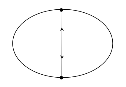
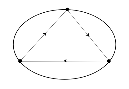
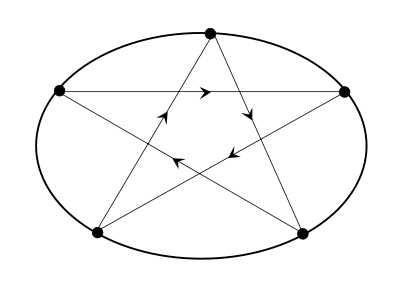
Examples of periodic orbits.
Note that this definition can be presented in terms of a lift of the transformation \(T\). That is, since \(\mathbb{R} / \mathbb{Z} \cong S^1\), consider a lift of \(T \colon S^1 \times I \to S^1 \times I\), and call it \(F \colon \mathbb{R} \times I \to \mathbb{R} \times I\). Then, a \((p,q)\)-periodic orbit is such that \(F^q(s_i, \theta_i) = (s_i + p, \theta_i)\).
Now, we wonder about the existence of such orbits. Using the fact that \(H\) is a generating function of \(T\), we can prove the following result making use of the results of section [sec:PO_cotangent]
For any \(q \geq 2\) and \(1 \leq p \leq \frac{1}{2} q\) coprime to \(p\), there exist two gometrically distinct \((p,q)\)-periodic orbits.
Proof
Consider the set \(M\) of inscribed \(q\)-gons of the table \(x_1, \ldots, x_q\), with \(x_i \in \partial \mathcal{M}\). Let \(H(x_1, \ldots, x_q) = \|x_1 - x_{q}\| + \|x_2 - x_1\| + \cdots + \|x_q - x_{q-1}\|\) be the perimeter length of a given \(q\)-gon, which is precisely the action of the periodic orbit of section [sec:action_po]. As we have discussed in the previous chapter, periodic orbits of \(T\) will correspond to critical points of \(H\) (recall that \(T\) is monotone). We will thus prove the existance of critical points of \(H\).
First, note that \(H\) is smooth outside of the set \(M_0 = \bigcup_i \{ x_i = x_{i+1}\}\). We now establish the existance of \((1,q)\)-periodic trajectories. Since \(M\) is compact, by Weierstrass’ theorem \(H\) attains its global maximum on it. Furthermore, this maximum cannot lie on \(M_0\), since any \(k\)-gon with \(k < q\) has a smaller perimeter than any proper \(q\)-gon.
In the general case, given \(p,q\), we define \(M\) as the set of inscribed star-shaped \(q\)-gons with \(p\) rotations around the table. Then, \(H\) has at least \(q\)-maxima in \(M\), obtained by a cyclic permutation of the vertices of the same geometrical polygon of maximal perimeter.
To show there are other critical points inside of \(M\), we use the min-max argument. That is, consider the set of curves inside \(M\) that connect two maximums of \(H\). Consider the minimum of \(H\) on each of these curves, and select the maximum of these minima. Then, this is also a critical point of \(H\) different from the maximum. Its existance is guaranteed by the fact that we do not need to come close to the boundary \(M_0\), since \(H\) increases as one moves away from \(M_0\).
The reason for considering \(p\) coprime to \(q\) is that this way we guarantee that the trajectory is not degenerate, that is, traversed by the billiard ball several times. ◻
Note that if \(p > q\), then the \(q\)-gons are the same but traversed in the reverse direction.
Finally, we remark that his result is equivalent to the Poincaré-Birkhoff theorem for twist maps in the particular case of the billiard map, but we have used a variational approach to prove it.
Length Spectrum
Having established the existence of periodic trajectories, we wonder about their lengths. This is related to the values that the periodic action \(H^{(p,q)}(x) = \sum_{i = 0}^{q-1} H(T^i(x))\) introduced in section [sec:action_po] can attain for a particular pair \((p,q)\). Recall that as discussed in said section, given a particular periodic orbit, this value is an invariant under symplectic changes of coordinates (up to an additive constant).
Consider the set \(\mathcal{O}^{(p,q)} = \{(s_i, \theta_i)\}\) of \((p,q)\)-periodic orbits. We assign to each \(O \in \mathcal{O}\) the value of its periodic action, \(H^{(p,q)}(O)\) (abusing notation).
The length spectrum of the billiard table \(\Gamma\) is the subset \(\mathcal{LS} \subset \mathbb{R}_+\) defined as \(\mathcal{LS}(\Gamma) = l \mathbb{N} + \bigcup_{(p,q)} \Lambda^{(p,q)} \mathbb{N}\), where \(l = \mathrm{length} (\Gamma)\) and \(\Lambda^{(p,q)} = \bigcup_{O \in \mathcal{O}^{(p,q)}} H(O)\) is the set of the lengths of all \((p,q)\)-periodic trajectories.
\(\Delta^{(p,q)} = \sup_{O , \bar O \in \mathcal{O}^{(p,q)}} \left| H^{(p,q)}(\bar O) - H^{(p,q)}(O)\right|\) is the supremum length difference.
This is basically the difference in length between the longest and shortest periodic orbit. We observe that \(\Delta^{(p,q)}\) has an interpretation in terms of the \(w\)-area of a certain region of phase space.
Let \(O, \bar O\) be 2 distinct \((p,q)\)-periodic orbits, \((s_0, \theta_0) \in O, \ (\bar s_0, \bar \theta_0) \in \bar O\). Let \(L_0\) be a curve from \((s_0, r_0)\) to \((\bar s_0, \bar r_0)\) contained in \(V\), and \(L_k = T^k(L_k)\). We consider \(B \subset V\) the domain enclosed between them. Then, \(\Delta^{(p,q)} \leq \mathrm{Area}_w (B)\).
Proof
Note that \(L_0\) and \(L_q\) have the same endpoints in \(V\). First assume that \(L_0, L_q\) have no topological crossings in \(V\). Then, \(\begin{gathered} \int_{L_{k+1}} \alpha - \int_{L_k} \alpha = \int_{L_k}(T^* \alpha - \alpha) = \int_{L_h} \mathrm{d} H = H(\bar s_k, \bar s_{k+1}) - H (s_k, s_{k+1}) \\ \implies \sum_{i = 0}^{q-1} \left( H(\bar s_i, \bar s_{i+1}) - H(s_i, s_{i+1})\right) = \int_{L_{q}} \alpha - \int_{L_0} \alpha = \int_{L_{q} - L_0} \alpha = \pm \int_{B} w, \end{gathered}\) where the sign \(\pm\) depends on the orientation of the closed path \(L_q-L_0\). It follows that \(\Delta^{(p,q)} = \int_B w = \mathrm{Area}_w(B).\) If the curve \(L_q\) or \(L_0\) have some topological crossing, then \(\Delta^{(p,q)} \leq \mathrm{Area}_w(B)\) because \(B\) has multiple connected components and the sign changes depends on the component. ◻
We will now state some results about \(\Delta^{(p,q)}\).
Consider \(\Gamma\) smooth, \(p\) fixed and periodic trajectories approaching \(\Gamma\) as \(q \to \infty\). Let \(L^{(p,q)}\) be the length of such a trajectory. Then, there exists a sequence \((l_k)_{k \geq 1}\) depending only on \(p\) and \(\Gamma\) such that \(L^{(p,q)} \asymp p \mathrm{Length}(\Gamma) + \sum_{k \geq 1} \frac{l_k}{q^{2k}}\) (the series is asymptotic to \(L^{(p,q)}\))
The asymptotic coefficients can be explicitly written in terms of the curvature \(\kappa(s)\). For example, \(l_1 = l_1(\Gamma, p) = - \frac{1}{24} \left( p \int_\Gamma \kappa^{\frac{2}{3}}(s) \mathrm{d}s \right)^3\).
In the analytic case, it turns out that \(\Delta^{(p,q)}\) are exponentially small. Indeed, the following proposition found in [@martin_length_2016] establishes this.
If \(\Gamma\) is analytic and \(p > 0\), then \(\exists K, \alpha > 0\) such that \(\Delta^{(p,q)} \leq K e^{-2 \pi \alpha \frac{q}{p}}\).
Finally, we would like to comment on the relevance of studying these lengths. First, it turns out that in some cases we can recover the geometry of the table from its length spectrum. This is due to the relation between \(\mathcal{LS}(\Gamma)\) and the spectrum of the Laplace operator in the billiard table. Furthermore, knowing the magnitude of \(\Delta^{(p,q)}\) is useful to understand how “far” the dynamics of rotation number \(\frac{p}{q}\) is from forming a smooth invariant circle, which is related to Aubrey-Mather theory. In near circular tables, \(\Delta^{(p,q)}\) decays exponentially fast, but in chaotic tables (such as the stadium) \(\Delta^{(p,q)}\) stays bounded away from 0.
References
- Ralph Abraham, Jerrold E Marsden, and Tudor Ratiu. Manifolds, tensor analysis, and applications. Vol. 75. Springer Science & Business Media, 2012.
- Alex Haro. “The Primite Function of an Exact Symplectomorphism”. PhD thesis. Universitat de Barcelona, July 1998.
- P. Martín, R. Ramírez-Ros, and A. Tamarit-Sariol. “Exponentially Small Asymptotic Formulas for the Length Spectrum in Some Billiard Tables”. en. In: Experimental Math- ematics 25.4 (Oct. 2016), pp. 416–440. issn: 1058-6458, 1944-950X. doi: 10.1080/10586458.2015.1076361. Pau Martín, Rafael Ramírez-Ros, and Anna Tamarit-Sariol. “On the length and area spectrum of analytic convex domains”. en. In: Nonlinearity 29.1 (Jan. 2016), pp. 198–231. issn: 0951-7715, 1361-6544. doi: 10.1088/0951-7715/29/1/198.
- K. Meyer and G. Hall. Introduction to Hamiltonian Dynamical Systems and the N-Body Problem. Applied Mathematical Sciences. Springer New York, 2013. isbn: 9781475740738. url.
- Eva Miranda et al. From Differential Topology to Symplectic Geometry and Beyond. Class notes. 2025.
- Serge Tabachnikov. Geometry and billiards. Vol. 30. American Mathematical Soc., 2005.
- Anna Tamarit Sariol, Rafael Ramírez Ros, and Pablo Martín De La Torre. “Singular phenomena in the length spectrum of analytic convex curves”. en. PhD thesis. Universitat Politècnica de Catalunya, July 2015. doi: 10.5821/dissertation-2117-95793.